Last month, a virtual fencing system for 4.0 livestock farming failed spectacularly: an entire herd crossed a dangerous area because the GPS collars lost signal. The control software did not record anomalies, but subsequent analysis revealed that the terrain's orography blocked the waves. This incident is not a simple technical failure; it is a lesson on how a poorly calibrated digital twin can put real assets at risk.
Error reconstruction: ArcGIS, MATLAB, and Blender on the stand 🛠️
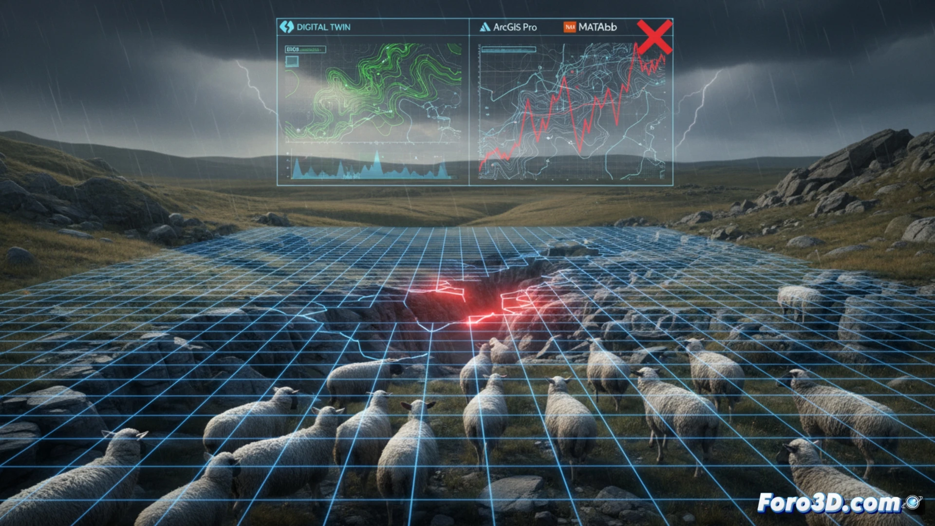
To understand the failure, a reverse workflow was applied. First, the digital elevation model of the terrain was imported into ArcGIS Pro with 3D Analyst to create an accurate mesh of the pasture and canyon. Second, GPS signal propagation was simulated in MATLAB using Ray Tracing, modeling the collars as transmitters and the base antenna as the receiver. The result was clear: in a depression with a steep slope, the signal reflected and attenuated until it disappeared, creating a 15-meter-wide dead zone. Finally, Blender was used to visualize the herd's path and the shadow zone, confirming that the original control software did not include this scenario in its digital twin.
Lessons for the next iteration of the virtual model 📐
The solution is not more hardware, but a more robust digital twin. The workflow must integrate wave propagation simulation (MATLAB) as a mandatory step before deploying collars. Additionally, ArcGIS Pro should feed the model with dynamic signal shadow maps, not just static topography. Finally, Blender allows visualizing these blind spots so that farmers understand the system's limits. A digital twin is not just a map; it is a simulator that must anticipate failures, not just record them after the disaster.
What lessons about managing limit states in digital twin simulations can we extract from a virtual fencing system that ignored a kinematic dead zone in its predictive model?
(PS: My digital twin is currently in a meeting, while I am here modeling. So technically, I am in two places at once.)